bloodstockR
Tattersalls
There are currently (as of 2016-04-15) 6 datasets with Tattersalls sales data, these are:
| Name | Sales included | Dim |
|---|---|---|
| tatts_2010 | feb, craven, guineas, july, oct_bk1, oct_bk2, oct_bk3, autumn_hit, breeders_flat, dec_yearlings, dec_foals, dec_mares | 7796 rows, 12 cols |
| tatts_2011 | feb, craven, breeze_up, july, oct_bk1, oct_bk2, oct_bk3, autumn_hit, breeders_flat, dec_yearlings, dec_foals, dec_mares | 6946 rows, 12 cols |
| tatts_2012 | dec_mares, dec_foals, dec_yearlings, autumn_hit, oct_bk3, oct_bk2, oct_bk1, july, guineas_hit, guineas, craven, feb | 7101 rows, 12 cols |
| tatts_2013 | feb, craven, guineas, guineas_hit, july, oct_bk1, oct_bk2, oct_bk3, oct_bk4, autumn_hit, dec_yearlings, dec_foals, dec_mares | 7192 rows, 12 cols |
| tatts_2014 | july, guineas, guineas_hit, craven, feb, oct_bk1, oct_bk2, oct_bk3, oct_bk4, autumn_hit, dec_yearlings, dec_foals, dec_mares | 7429 rows, 12 cols |
| tatts_2015 | feb, craven, guineas, guineas_hit, july, oct_bk1, oct_bk2, oct_bk3, oct_bk4, autumn_hit | 5389 rows, 12 cols |
There is a function to collect data from sales not included in the package, see here.
To load a dataset:
data(tatts_2010)Each of the 5 datasets have the same 12 variables, year, sale, sale_name, lot_no, horse, sex, color, sire, dam, seller, buyer, price, as can be seen in the table above, the same sales take place each year.
Some Analysis
It is easy to combine the 5 datasets, such as:
data(tatts_2010, tatts_2011, tatts_2012, tatts_2013, tatts_2014)

# combine all 5 datasets into one large dataset
tattersalls <- rbind(tatts_2010, tatts_2011, tatts_2012, tatts_2013, tatts_2014)
# clean workspace
rm(tatts_2010, tatts_2011, tatts_2012, tatts_2013, tatts_2014)
The new tattersalls dataset has 36464 rows and 12 columns, the sale_name variable can serve as an individual sale (so it includes the year of the sale, eg. feb_2010), while the sale variable will match across multiple years.
Loading other libraries dplyr and ggplot2 we can quickly analyse data:
library(dplyr)
library(ggplot2)
The average price of lots in each sale across multiple years:
sale_summaries <- tattersalls %>%
    group_by(sale, year) %>%
    summarise(n = n(),
              mean = mean(price, na.rm=T))

ggplot(sale_summaries, aes(x=year, y=mean)) +
    geom_bar(stat="identity", fill="#D9220F") +
    theme_bw() +
    theme(text = element_text(size=10)) +
    facet_wrap(~sale)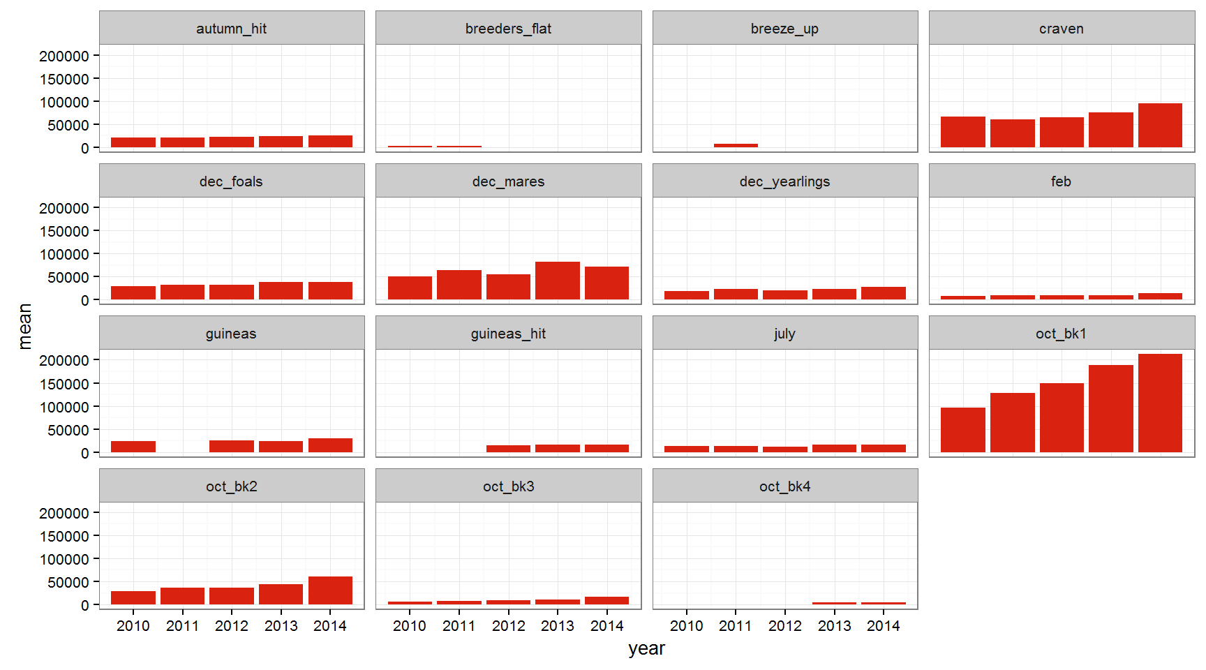
One thing stands out immediately from the plots above, don’t go to October Book 1 unless you have deep pockets, the average price paid has more than doubled from 96,001 Guineas in 2010 to 212,637 Guineas in 2014. October Book 2 has also (unsurprisingly) seen a small increase in average price paid over the same period. The Craven sale has also seen a small increase over recent years, but prices are in other sales appear to be quite consistent.
We can also find the 20 sires with the highest average price over the 5 years:
tattersalls %>%
    group_by(sire) %>%
    summarise(n = n(),
              mean = mean(price, na.rm=T),
              sd = sd(price, na.rm=T),
              min = min(price, na.rm=T),
              max = max(price, na.rm=T)) %>%
    filter(n >= 50) %>%
    arrange(desc(mean)) %>%
    head(20)
## Source: local data frame [20 x 6]
##
## sire n mean sd min max
## (chr) (int) (dbl) (dbl) (dbl) (dbl)
## 1 galileo (ire) 572 211314.35 409799.91 800 5000000
## 2 sea the stars (ire) 182 199763.89 150603.40 6000 650000
## 3 danehill (usa) 52 124195.56 379083.76 2000 2400000
## 4 new approach (ire) 238 108774.87 110347.56 2500 600000
## 5 montjeu (ire) 326 105223.87 156474.57 800 850000
## 6 dubawi (ire) 372 97881.49 169775.01 800 1600000
## 7 sadler's wells (usa) 156 96807.09 201949.61 1000 1700000
## 8 oasis dream (gb) 594 94710.82 143449.05 800 1100000
## 9 monsun (ger) 84 93459.70 109112.35 2000 600000
## 10 dansili (gb) 434 84944.14 184443.84 800 2700000
## 11 fastnet rock (aus) 154 83655.46 84648.97 4000 540000
## 12 raven's pass (usa) 140 81896.75 104884.44 800 800000
## 13 danehill dancer (ire) 499 80129.26 227178.69 800 4000000
## 14 invincible spirit (ire) 653 80056.97 128397.23 800 2100000
## 15 lope de vega (ire) 83 75378.38 98854.63 1000 650000
## 16 pivotal (gb) 630 72477.19 225981.29 800 4700000
## 17 lawman (fr) 281 70083.76 301039.09 800 4500000
## 18 shamardal (usa) 478 69765.14 118171.36 800 1700000
## 19 poet's voice (gb) 105 69760.64 104033.18 3500 700000
## 20 rip van winkle (ire) 130 68780.37 65442.26 4000 400000Sea The Stars is top of the list, his progeny costing a cool 224,100 Guineas on average, Galileo is a very close second, with a large drop down, of almost 100,000 Guineas, to Danehill. Perhaps more interesting than Sea The Stars topping Galileo is the standard deviation of their prices, Sea The Stars with a much smaller sd perhaps suggests buyers believe his progeny will prove to be successful (see Taghrooda), but are still showing some restraint and aren’t quite willing to part with the big sums seen with Galileo, whose most expensive sale fetched 9 times the most expensive Sea The Stars sale.
It’s also possible to look at the buyers or agents with the highest average price paid over the 5years.
tattersalls %>%
    group_by(buyer) %>%
    summarise(n = n(),
              mean = mean(price, na.rm=T),
              sd = sd(price, na.rm=T),
              min = min(price, na.rm=T),
              max = max(price, na.rm=T)) %>%
    filter(n >= 50) %>%
    arrange(desc(mean)) %>%
    head(20)
## Source: local data frame [20 x 6]
##
## buyer n mean sd min max
## (chr) (int) (dbl) (dbl) (dbl) (dbl)
## 1 demi o'byrne 51 342019.61 264811.14 6000 1300000
## 2 john ferguson bloodstock 314 215003.18 296659.68 25000 4000000
## 3 j warren bloodstock 86 176343.02 146367.91 16500 680000
## 4 shadwell estate company 234 173025.64 135849.13 35000 1100000
## 5 c gordon-watson bloodstock 281 149810.68 196409.25 800 1700000
## 6 david redvers bloodstock 202 121936.63 223385.67 5000 2500000
## 7 john warren bloodstock 93 118645.16 95735.10 11000 600000
## 8 badgers bloodstock 53 118452.83 159747.10 10000 800000
## 9 dwayne woods 59 95652.54 79130.74 3000 450000
## 10 mrs a skiffington 63 81595.24 80855.60 3000 400000
## 11 blandford bloodstock 452 80300.00 103073.80 800 925000
## 12 jeremy brummitt 67 78544.78 85540.03 6500 475000
## 13 anthony stroud bloodstock 242 75130.17 74083.30 800 425000
## 14 richard frisby bloodstock 90 72338.89 83634.50 2000 370000
## 15 brian grassick bloodstock 52 70176.92 61604.80 2200 360000
## 16 peter & ross doyle bloodstock 382 68610.47 76552.10 800 800000
## 17 hugo merry bloodstock 141 68357.45 92076.88 1700 675000
## 18 stephen hillen bloodstock 171 67578.95 167784.40 3000 2100000
## 19 sackvilledonald 191 66107.33 58515.52 2500 460000
## 20 kern/lillingston association 139 57712.23 70722.67 3800 460000Demi O’Byrne (an agent associated with Coolmore) isn’t as active as others in the top 5, with just 50 purchases, but the average price he pays is almost double that of John Ferguson (links with Godolphin).